What Baby Names are In and Out of Fashion?

Using open data to summarize baby names over time

Open Data of Baby Names

Open Data Buffalo is a great resource and initiative to make datasets open and available to the public.

My partner works at a Children’s hospital and is convinced of trending baby names. Well, I said to her let’s see what the data says!

So I ventured out into the world wide web and found a dataset called:

Baby Names: Beginning 2007

New York State (NYS) Baby Names are aggregated and displayed by the year, county, or borough where the mother resided as stated on a New York State or New York City (NYC) birth certificate. The frequency of the baby name is listed if there are 5 or more of the same baby name in a county outside of NYC or 10 or more of the same baby name in a NYC borough.

library(jsonlite)
library(RSocrata)
suppressMessages(library(tidyverse))

baby_names <- RSocrata::read.socrata("https://health.data.ny.gov/resource/jxy9-yhdk.json",app_token = read_json('.apptoken')[['token']])

baby_names %>% glimpse()

Rows: 87,899
Columns: 5
$ year       <chr> "2007", "2007", "2007", "2007", "2007", "2007", "2007", "20…
$ first_name <chr> "ZOEY", "ZOEY", "ZOEY", "ZOEY", "ZOE", "ZOE", "ZOE", "ZOE",…
$ county     <chr> "KINGS", "SUFFOLK", "MONROE", "ERIE", "ULSTER", "WESTCHESTE…
$ sex        <chr> "F", "F", "F", "F", "F", "F", "F", "F", "F", "F", "F", "F",…
$ name_count <chr> "11", "6", "6", "9", "5", "24", "13", "55", "15", "6", "14"…

This dataset is already tidy: One row per observation (first_name or baby name) and one column per variable (e.g. the number of observed names in a county with the given gender on the birth certificate).

I first check a few data quality characteristics such as missingness and number of unique things in each column:

purrr::map_dfr(baby_names,~{sum(is.na(.x))})

# A tibble: 1 × 5
   year first_name county   sex name_count
  <int>      <int>  <int> <int>      <int>
1     0          0      0     0          0

purrr::map_dfr(baby_names,~{n_distinct(.x)})

# A tibble: 1 × 5
   year first_name county   sex name_count
  <int>      <int>  <int> <int>      <int>
1    14       2320    123     2        244

The baby_names dataset requires initial preprocessing

Now we need to transform our dataset by first converting columns to the appropriate data types:

baby_names_transformed <- 
    baby_names %>% 
    mutate(
        year = as.integer(year),
        first_name = factor(first_name),
        county = factor(county),
        sex = factor(sex,levels=c("M","F"),labels=c("Male","Female")),
        name_count = as.integer(name_count)
    )

baby_names_transformed %>% summary()

      year        first_name        county          sex          name_count    
 Min.   :2007   EMMA   :  528   Kings  : 5715   Male  :46737   Min.   :  5.00  
 1st Qu.:2010   OLIVIA :  503   KINGS  : 4957   Female:41162   1st Qu.:  6.00  
 Median :2014   LOGAN  :  488   Suffolk: 4159                  Median : 11.00  
 Mean   :2013   MASON  :  475   SUFFOLK: 4005                  Mean   : 17.77  
 3rd Qu.:2017   LIAM   :  471   Queens : 3868                  3rd Qu.: 19.00  
 Max.   :2020   JACOB  :  465   Nassau : 3804                  Max.   :297.00  
                (Other):84969   (Other):61391                                  

After the data transformation, we see that counties are specified in different cases. We should revise this so county (and also first_name) are in one type of case such as title case:

baby_names_transformed <- 
    baby_names_transformed %>% 
    mutate(
        first_name = as.character(first_name) %>% stringr::str_to_title() %>% factor(),
        county = as.character(county) %>% stringr::str_to_title() %>% factor()
    )

baby_names_transformed %>% summary()

      year        first_name            county          sex       
 Min.   :2007   Emma   :  528   Kings      :10672   Male  :46737  
 1st Qu.:2010   Olivia :  503   Suffolk    : 8164   Female:41162  
 Median :2014   Logan  :  488   Nassau     : 7352                 
 Mean   :2013   Mason  :  475   Queens     : 7244                 
 3rd Qu.:2017   Liam   :  471   Westchester: 5844                 
 Max.   :2020   Jacob  :  465   Erie       : 5382                 
                (Other):84969   (Other)    :43241                 
   name_count    
 Min.   :  5.00  
 1st Qu.:  6.00  
 Median : 11.00  
 Mean   : 17.77  
 3rd Qu.: 19.00  
 Max.   :297.00  
                 

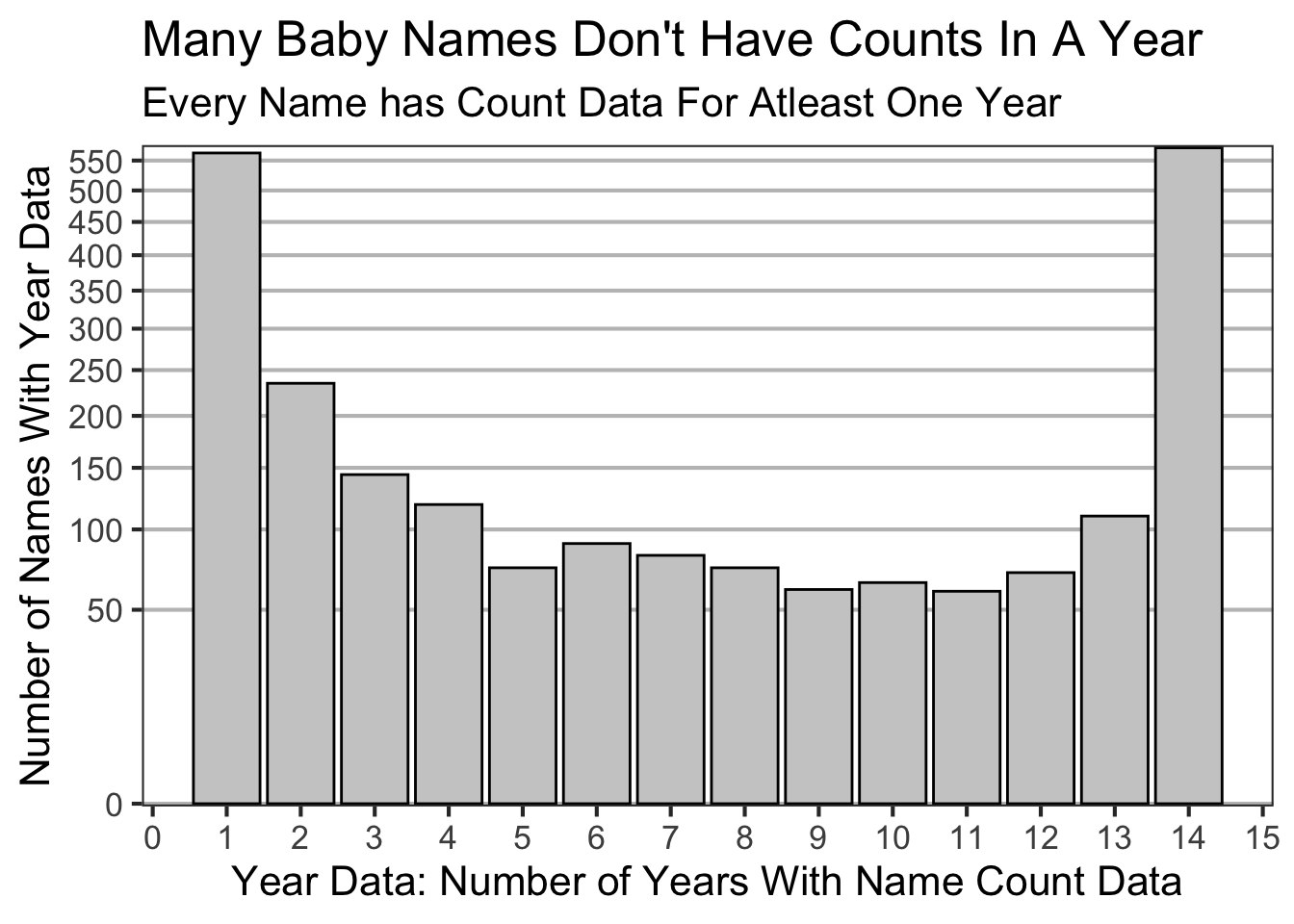
Many Baby Names Don’t Have Counts In A Year

My next data quality question is how many names have data each year?

theme_set(theme_bw(base_size = 16))

baby_names_transformed %>% 
    summarize(n_years = n_distinct(year),.by=c(first_name)) %>% 
    summarize(n_names = n_distinct(first_name),.by=n_years) %>% 
    ggplot(aes(n_years,n_names)) +
    geom_bar(color="black",fill = "gray80",stat = "identity") +
    scale_x_continuous(breaks = scales::pretty_breaks(14)) +
    scale_y_continuous(expand = c(0,0.1),
                       trans="sqrt",breaks = scales::pretty_breaks(10)) +
    labs(x="Year Data: Number of Years With Name Count Data",
         y="Number of Names With Year Data",
         title="Many Baby Names Don't Have Counts In A Year",
         subtitle="Every Name has Count Data For Atleast One Year") +
    theme(
        panel.grid.major.y = element_line(color="gray75"),
        panel.grid.minor.y = element_blank(),
        panel.grid.major.x = element_blank(),
        panel.grid.minor.x = element_blank()
    )

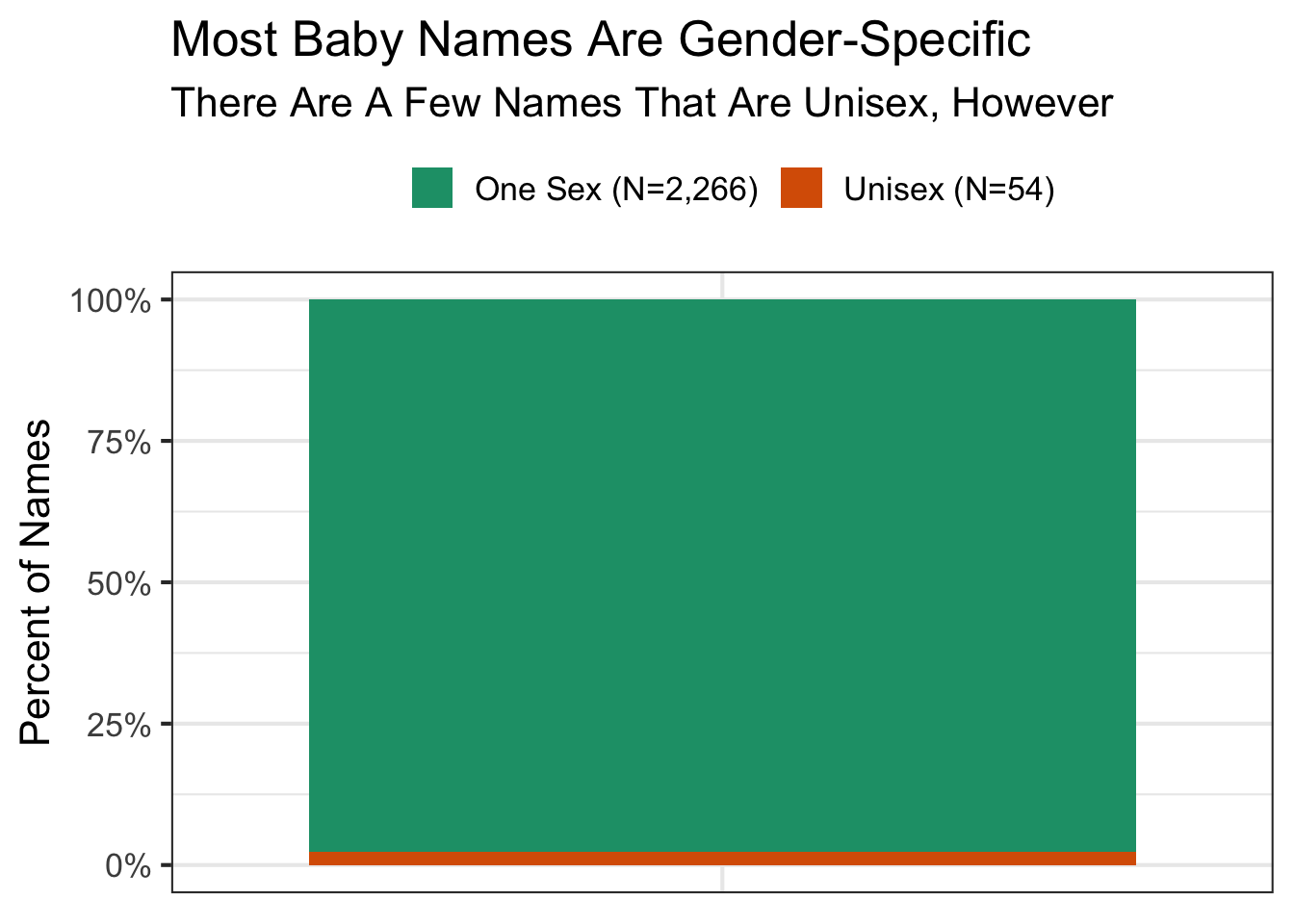
Most Baby Names Are Gender-Specific

Another question is are there many names that are unisex i.e. male and female names?

tmp <- 
    baby_names_transformed %>% 
    summarize(n_sex = n_distinct(sex),
              unisex = n_sex==2,onesex = n_sex==1,
              .by=c(first_name)) %>% 
    summarize(`Unisex` = sum(unisex),`One Sex`=sum(onesex))

tmp %>% 
    pivot_longer(cols = everything()) %>% 
    mutate(label = glue::glue("{name} (N={scales::comma(value)})")) %>% 
    ggplot(aes(factor(1),value,fill=label)) +
    geom_bar(stat="identity",position = "fill") +
    scale_fill_brewer(palette = "Dark2") +
    scale_y_continuous(labels = scales::percent) +
    guides(fill=guide_legend(title=NULL)) +
    labs(x=NULL,y="Percent of Names",title="Most Baby Names Are Gender-Specific",subtitle = "There Are A Few Names That Are Unisex, However") +
    theme(
        axis.ticks.x = element_blank(),
        axis.text.x = element_blank(),
        legend.position = "top"
    )

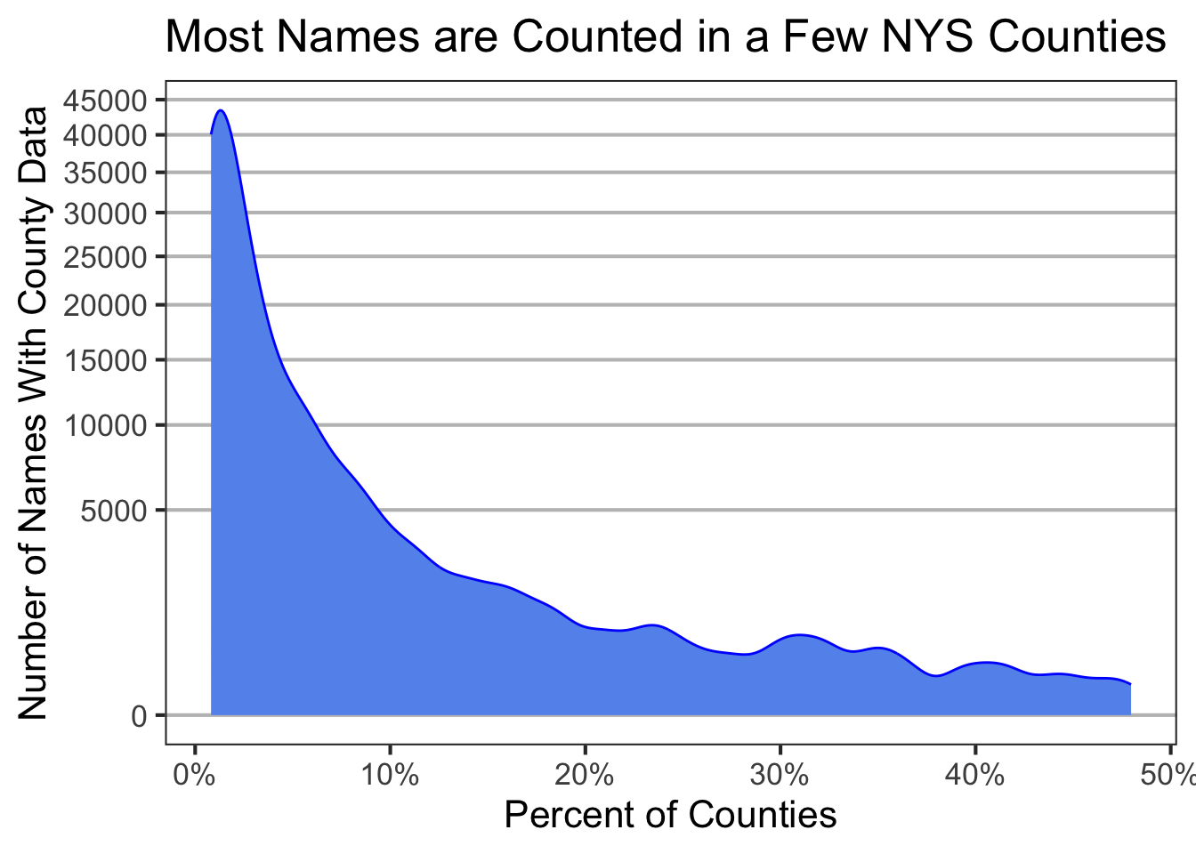
Most Baby Names are Counted in a Few NYS Counties

My last data quality question is how many baby names have data across counties?

baby_names_transformed %>% 
    summarise(n_counties = n_distinct(county),.by=first_name) %>% 
    bind_cols(
        summarise(baby_names,total_counties = n_distinct(county))
    ) %>% 
    mutate(
        freq_counties = n_counties / total_counties
    ) %>% 
    ggplot(aes(freq_counties,y=after_stat(count))) +
    geom_density(bw="nrd",color="blue",fill="cornflowerblue") +
    scale_x_continuous(labels = scales::percent) +
    scale_y_sqrt(breaks = scales::pretty_breaks(15)) +
    labs(x="Percent of Counties",y="Number of Names With County Data",
         title="Most Names are Counted in a Few NYS Counties") +
    theme(
        panel.grid.major.y = element_line(color="gray75"),
        panel.grid.minor.y = element_blank(),
        panel.grid.major.x = element_blank(),
        panel.grid.minor.x = element_blank()
    )

After transforming the dataset and checking data quality, we see that:

1. Baby names are sparsely annotated across counties
2. Baby names are, generally, specific to a year or are observed across all years
3. There are a few baby names that are not gender-specific.

What are the trending baby names in NYS?

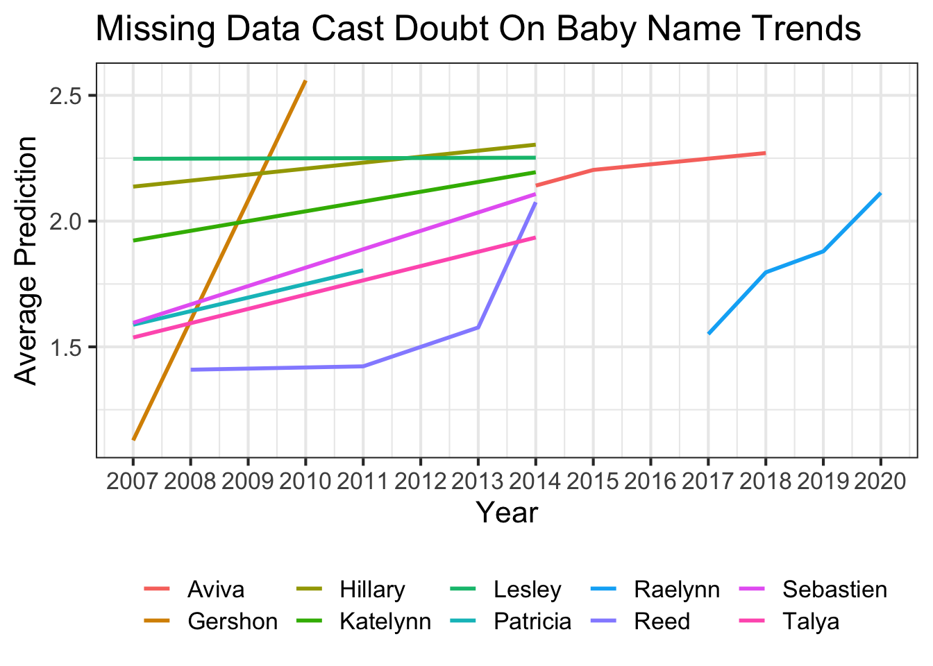
I want to ask the question what are the trending baby names in NYS? My question is not specific to the gender or county. Also, my question wants to consider all the baby names in the dataset as possible influencing factors in which baby names are trending. Because of the missing count data, we should use a model to estimate the trend based on the available data. The model we will use is a generalized additive model (GAM) to predict the Poisson distribution count of the baby name. *

*I heavily referenced https://fromthebottomoftheheap.net/2021/02/02/random-effects-in-gams/

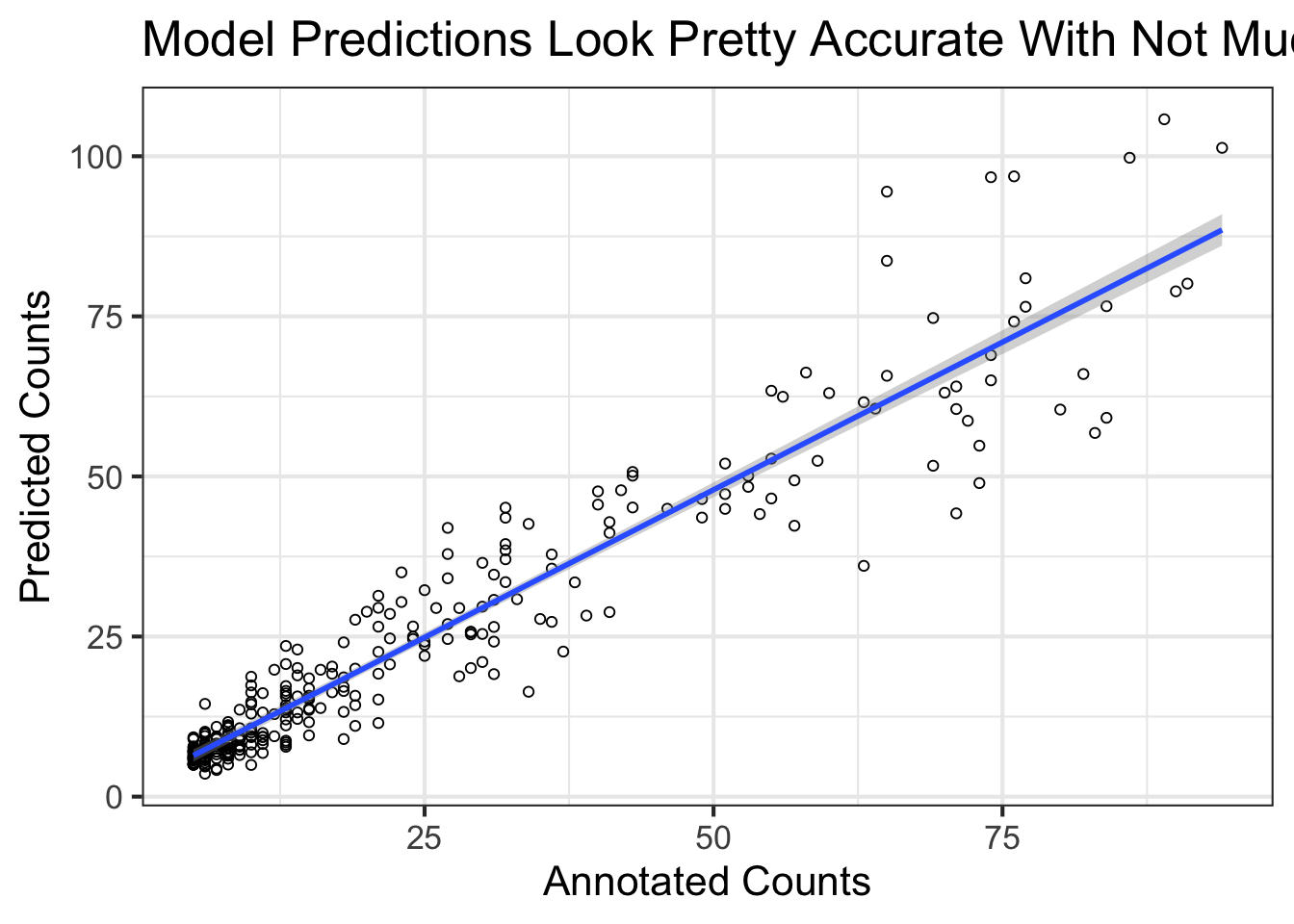
We can estimate baby name trends using generalized additive models

Let’s do a small example first. My subquestion is, is the baby name Charlotte trending over time irrespective of other factors?

library(mgcv)

Loading required package: nlme

Attaching package: 'nlme'

The following object is masked from 'package:dplyr':

    collapse

This is mgcv 1.8-42. For overview type 'help("mgcv-package")'.

tmp <- 
    baby_names_transformed %>% 
    filter(first_name=="Charlotte")

form <- as.formula(glue::glue("name_count ~ s(year) + county:year"))
fit <- mgcv::gam(form,
                family="poisson",
                data=tmp,method = "GACV.Cp")

tmp %>% 
    bind_cols(.pred = fit$fitted.values) %>% 
    ggplot(aes(name_count,.pred)) +
    geom_point(shape=21) +
    geom_smooth(formula = 'y ~ x',method="lm") +
    labs(x="Annotated Counts",y="Predicted Counts",title="Model Predictions Look Pretty Accurate With Not Much Bias")

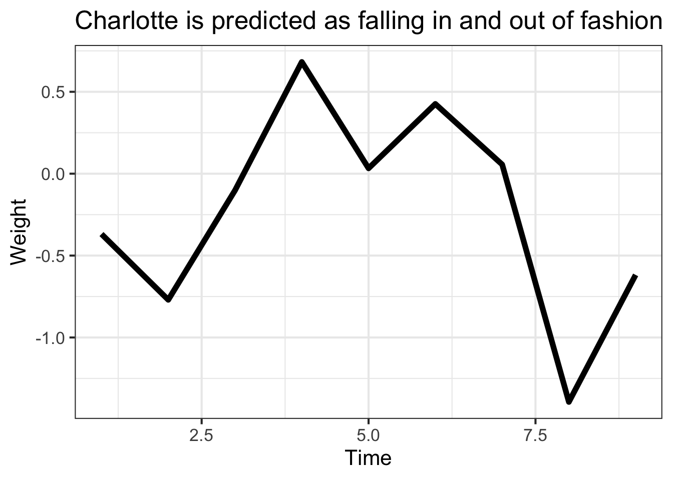
coefs_ <- fit$coefficients[str_detect(names(fit$coefficients),"s\\(year\\)")] %>% unname()
tibble(
    year = seq_along(coefs_),
    coef = coefs_
) %>% 
    ggplot(aes(year,coef)) +
    geom_line(linewidth=2) +
    labs(x="Time",y="Weight",title="Charlotte is predicted as falling in and out of fashion")

GAMs allow for estimating trends given “random” naming patterns across NYS counties over time

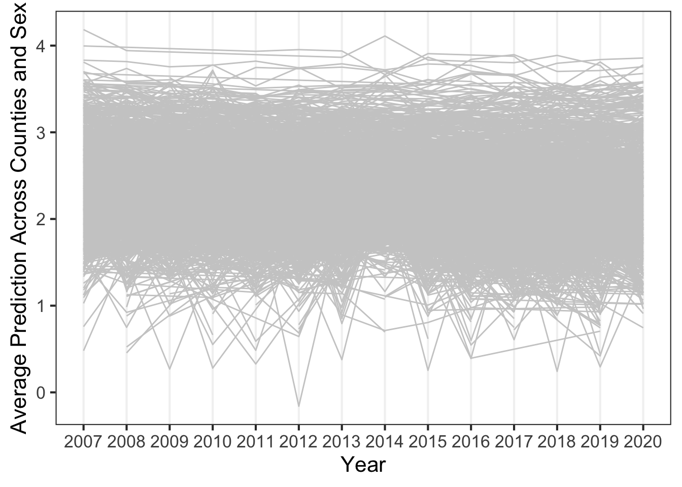
If we want to consider all names, we need to specify the name as a random effect and the trend line as a random slope between the name and the year:

(form <- as.formula(glue::glue("name_count ~ s(first_name, bs = 're') + s(first_name, year, bs = 're') + county:year + sex:year")))

name_count ~ s(first_name, bs = "re") + s(first_name, year, bs = "re") + 
    county:year + sex:year

We can use this formula in our model to get the trends of the baby names over time (Note: we switch from gam to bam so that we can fit the model faster using method = ‘fREML’):

tmp <- 
    baby_names_transformed

if(file.exists(paste0(here::here(),"/baby_name_gam_full.rds"))){
    fit <- readr::read_rds(paste0(here::here(),"/baby_name_gam_full.rds"))
}else{
    system.time(fit <- mgcv::bam(form,
                 family = "poisson",
                 data = tmp,
                 discrete = TRUE))
    readr::write_rds(fit,paste0(here::here(),"/baby_name_gam_full.rds"))
}

Now we combine the predicted baby name counts to the original data:

(data_pred <- 
        bind_cols(tmp,
                  as.data.frame(predict(fit,
                                        new_data = tmp,
                                        se.fit = TRUE))) %>% 
        tibble())

# A tibble: 87,899 × 7
    year first_name county      sex    name_count   fit se.fit
   <int> <fct>      <fct>       <fct>       <int> <dbl>  <dbl>
 1  2007 Zoey       Kings       Female         11  3.58 0.0206
 2  2007 Zoey       Suffolk     Female          6  3.09 0.0207
 3  2007 Zoey       Monroe      Female          6  2.39 0.0210
 4  2007 Zoey       Erie        Female          9  2.59 0.0209
 5  2007 Zoe        Ulster      Female          5  1.68 0.0200
 6  2007 Zoe        Westchester Female         24  3.15 0.0155
 7  2007 Zoe        Bronx       Female         13  3.69 0.0153
 8  2007 Zoe        New York    Female         55  3.61 0.0153
 9  2007 Zoe        Nassau      Female         15  3.45 0.0153
10  2007 Zoe        Erie        Female          6  3.09 0.0155
# ℹ 87,889 more rows

And we can now plot predicted baby name trends over time:

pred_baby_names <- 
    data_pred %>% 
    summarize(avg_pred = mean(fit),.by=c(first_name,year))

pred_baby_names %>% 
    ggplot(aes(year,avg_pred,group=first_name)) +
    geom_line(show.legend = F,color="gray80") +
    scale_x_continuous(breaks = scales::pretty_breaks(14)) +
    labs(x="Year",y="Average Prediction Across Counties and Sex") +
    theme(
        panel.grid.major.y = element_blank(),
        panel.grid.minor.y = element_blank(),
        panel.grid.major.x = element_line(color="gray95"),
        panel.grid.minor.x = element_blank()
    )

Now we have trend estimates for baby names over time considering the naming variability across counties, gender, and years.

GAM estimates offer robust baby name trends, but still need to consider data missingness

We can now ask the question what are the top trending baby names in NY?

(top_10_baby_names <- 
    pred_baby_names %>% 
    summarise(cor = cor(year,avg_pred,method="spearman"),.by = first_name) %>% 
    slice_max(order_by = cor,n = 10,with_ties = F))

# A tibble: 10 × 2
   first_name   cor
   <fct>      <dbl>
 1 Reed           1
 2 Aviva          1
 3 Raelynn        1
 4 Talya          1
 5 Sebastien      1
 6 Patricia       1
 7 Lesley         1
 8 Katelynn       1
 9 Hillary        1
10 Gershon        1

pred_baby_names %>% 
    filter(first_name %in% top_10_baby_names$first_name) %>% 
    ggplot(aes(year,avg_pred,color=first_name)) +
    geom_line(linewidth=1) +
    scale_x_continuous(breaks = scales::pretty_breaks(14)) +
    labs(x="Year",y="Average Prediction",title="Missing Data Cast Doubt On Baby Name Trends") +
    guides(color=guide_legend(title=NULL)) +
    theme(
        legend.position = "bottom"
    )

Looks like I need to add a variable for the name attributing how many years worth of count data it has as well as if it was a name in 2019 or 2020.

(pred_baby_names <- 
    pred_baby_names %>% 
    left_join(
        data_pred %>% 
        summarise(n_years = n_distinct(year),prop_years = n_years/14,
                  recent = any(year %in% c(2019,2020)),.by=first_name),
        by = "first_name"
    ))

# A tibble: 16,166 × 6
   first_name  year avg_pred n_years prop_years recent
   <fct>      <int>    <dbl>   <int>      <dbl> <lgl> 
 1 Zoey        2007     2.91      14      1     TRUE  
 2 Zoe         2007     3.21      14      1     TRUE  
 3 Zissy       2007     2.50      14      1     TRUE  
 4 Zion        2007     3.02      14      1     TRUE  
 5 Zev         2007     3.00      14      1     TRUE  
 6 Zara        2007     2.79      14      1     TRUE  
 7 Zaire       2007     2.68      13      0.929 TRUE  
 8 Zackary     2007     1.87       2      0.143 FALSE 
 9 Zachary     2007     2.23      14      1     TRUE  
10 Yusuf       2007     2.26      13      0.929 TRUE  
# ℹ 16,156 more rows

Filtering our GAM estimates can give more reliable top trending baby names in NYS

Now we can ask what are the top 10 trending baby names that are recently popular?

(top_10_recent_baby_names <- 
    pred_baby_names %>% 
    filter(recent & prop_years>.5) %>% 
    summarise(cor = cor(year,avg_pred,method="spearman"),.by = first_name) %>% 
    slice_max(order_by = cor,n = 10,with_ties = F))

# A tibble: 10 × 2
   first_name   cor
   <fct>      <dbl>
 1 Tyler      0.982
 2 Joshua     0.974
 3 Alyssa     0.965
 4 Nicholas   0.947
 5 Aiden      0.947
 6 Jacob      0.925
 7 Kaylee     0.921
 8 Aidan      0.912
 9 Abigail    0.912
10 Ryan       0.908

pred_baby_names %>% 
    filter(first_name %in% top_10_recent_baby_names$first_name) %>% 
    mutate(first_name = factor(first_name,top_10_recent_baby_names$first_name)) %>% 
    ggplot(aes(year,avg_pred,color=first_name)) +
    geom_line(linewidth=1) +
    scale_x_continuous(breaks = scales::pretty_breaks(14)) +
    labs(x="Year",y="Average Prediction",title="Top 10 Trending Names") +
    guides(color=guide_legend(title=NULL)) +
    theme(
        legend.position = "top"
    )

pred_baby_names %>% 
    filter(first_name %in% top_10_recent_baby_names$first_name) %>% 
    mutate(first_name = factor(first_name,top_10_recent_baby_names$first_name)) %>% 
    ggplot(aes(year,avg_pred,color=first_name)) +
    geom_line(linewidth=1,show.legend = FALSE) +
    scale_x_continuous(breaks = scales::pretty_breaks(14)) +
    facet_wrap(~first_name,ncol=3) +
    labs(x="Year",y="Average Prediction",title="Top 10 Baby Trending Names") +
    theme(
        axis.text.x = element_text(angle=90,vjust=1,hjust=1)
    )

So there we go! This seems accurate, as a top trending baby name is Nicholas and my nephew’s name (born in 2018) is Aiden 🤓

And here is a summary table with the trending baby names in order:

pred_baby_names %>% 
    summarise(cor = cor(year,avg_pred,method="spearman"),
              .by = c(first_name,recent,prop_years)) %>% 
    arrange(desc(recent),desc(prop_years),desc(cor)) %>% 
    DT::datatable()

This was a fun post and exploration of trending baby names in NYS. If you made it this far, I hope you enjoyed reading 😁